SQL Tutorial
Friendly tips to help you learn SQL
select 💝 from wagon_team;
This tip builds on the analysis of a 🍌banana store🍌 introduced in Summarizing Data in SQL tip.
Comparing two numerical measures is very important as we try to summarize our data. Though the math becomes more complicated, SQL can still handle it. For example, we might be nervous that if people have to wait too long, they end up spending less money when they get to the front of the line. To get a rough idea of the relationship between wait-time and revenue, we might write a query very similar to the histogram one:
These queries give us some insight into the join distribution (plug: Wagon makes charts like these super easy to generate). We might also be interested in more statistical measurements like covariance or correlation. Most of the popular SQL implementations have these statistics built in, so for example in Postgres/Redshift we can write:
Postgres has all kinds of cool aggregate functions, including linear regressions - right in our SQL query!
Read these SQL tips to learn more:
This tip builds on the analysis of a 🍌banana store🍌 introduced in Summarizing Data in SQL tip.
It’s often useful to have a rough idea of the distribution of the data in a table or query result. Generating a histogram is a great way to understand that distribution. What’s the distribution of revenue per purchase at the banana stand? I mean, how much could a banana cost? We might (naively) write a query like:
It’s likely this query will return far too many rows to eyeball the revenue distribution (1 row per distinct price). Instead, we’d like to group revenue values together into buckets so that we can understand the shape of the data. We might be interested in the number of banana purchases which generated between $0 to $5, $5 to $10, etc. There’s no “correct” number of buckets to use, it’s a choice we can make and experiment with to get a better understanding of the distribution. Probably 1000 buckets is too many, but 2 is too few. A reasonable rule of thumb is to use somewhere around 20 buckets. Our query will specify the width of the bucket, rather than the total number. The larger the width, the fewer buckets we’ll end up with.
This is a simple, but tricky query that will generate a histogram for us. It rounds each revenue data point down to the nearest multiple of 5 and then groups by that rounded value. It has one failing in that if we have no data in a bucket (e.g. no purchases of 55 to 60 dollars), then that row will not appear in the results. We can fix that with a more complex query, but let’s skip it for now. In order to choose our bucket size, it helps to first calculate the min/max values so we know how many buckets we would end up with. If we want the buckets to have slightly nicer labels, we can format the labels with a query like:
Read these SQL tips to learn more:
This tip builds on the analysis of a 🍌banana store🍌 introduced in Summarizing Data in SQL tip.
How long do people wait for their tasty banana orders? Using basic SQL we can compute average wait time, but if the distribution is skewed away from normal (as many internet-driven (and banana?) distributions often are), this may not give us a complete picture of how long most people are waiting. In addition to computing the average, we might (and should) ask, what are the 25th, 50th, 75th percentiles of wait-time, and how does that number vary day to day?
Many databases (including Postgres 9.4, Redshift, SQL Server) have built in percentile functions. Here’s an example using the function percentile_cont which is a window function that computes the percentile of wait-time, split (pun intended!) by day:
The structure of the percentile_cont is similar to other window functions: we specify how to order the data, how to group it - and the database does the rest. If we wanted to add more dimensions to our query (e.g. time of day), we’d add them to the partition and group by clause.
If our database doesn’t support percentile_cont (sorry MySQL, Postgres < 9.4), the query is more complicated, but fear not, still possible! The challenge is to order the rows by increasing wait-time (per date of course) and then pick out the middle value (for median). In MySQL, we can use local variables to keep track of the order, and in Postgres, we can use the row-number function. Here’s the Postgres version:
Read these SQL tips to learn more:
How quickly can you understand data from your database? Excel croaks at ten thousands rows, R is difficult to run on a cluster, and your eye certainly can’t summarize large tables. SQL to the rescue!
Summary statistics are the fastest way to learning about your dataset. Are there outliers? How does the distribution look? What are the relationships hiding inside the rows and columns? You’ll always want to ask these questions when faced with a new dataset. SQL (an uninspired acronym for Structured Query Language) is the native language for database computation. Many summary methods are available as built in SQL functions in modern databases and more complex measures can be implemented directly in SQL as well.
In this post, we’ll walk through 4 ways to summarize your dataset in SQL so you can run it directly on your database.
Here’s a relatable example: suppose we work in a 🍌banana stand’s🍌 back office and we analyze banana data.
With just a few SQL commands, we’ll be able to calculate the basic stats: count, distinct, sum, average, variance, … If we have a table of banana transactions, let’s calculate the total number of customers, unique customers, number of bananas sold, as well as total and average revenue per day:
This should be a familiar SQL pattern (and if not, come to the next free Wagon SQL class!). With just one query, we can calculate important aggregations over very large datasets. If we dress it up with a few where statements or join with customer lookup tables, we can quickly and effectively slice and dice our data. Unfortunately, there are some tricky questions that can’t be answered with the regular SQL functions alone.
Read these SQL tips to learn more:
Timestamps are great for debugging logs. But for analysis, we want to group by day, week, and month.
Timestamps look like this: 07/04/1776 00:28:39.682, but you’d rather see “July 4, 1776”, “July 1776” or “Q3 - 1776” 🇺🇸. Let’s clean up those messy timestamps in SQL!
Postgres & Redshift
In Postgres & Redshift, the to_char function is handy for formatting dates. It takes two arguments: a timestamp and the output format pattern. For example, the following returns “July 04, 1776”:
select to_char('07/04/1776 00:28:39.682'::timestamp, 'Month DD, YYYY');
The next SQL statement returns “Q3 - 1776”, by concatenating “Q” to the quarter and year from the to_char function.
select 'Q' || to_char('07/04/1776 00:28:39.682'::timestamp, 'Q - YYYY');
Pro Tip: Use to_char to format numbers too! See all the possibilities in the official docs.
MySQL
In MySQL, the date_format function will make those timestamps prettier. Here’s how to make ‘1776-07-04 00:28:39.682’ look like “July 4, 1776”:
select date_format('1776-07-04 00:28:39.682', '%M %e, %Y');
Learn More
- Official
to_charanddate_formatdocs - Date format by country (Wikipedia)
What’s the difference between a database, schema, and a table? Let’s break it down.
In relational databases, data is organized in a hierarchy, like files and folders. Databases have schemas. Schemas have tables. Tables have columns.
The standard flow is you connect to a database, browse schemas, and query a table’s columns. There are a few differences for this organization for Postgres, Redshift, and MySQL so here are some tips to navigating your database.
Postgres & Redshift
In Postgres and Redshift, you connect to a single database and can only access schemas and their tables within that database.
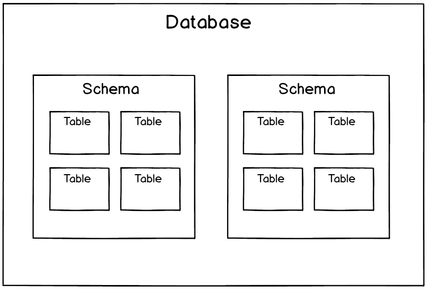
For example, in Wagon’s demo database, there is a schema named dvd containing tables such as products, orders, and customers.
To query one of these tables, you need to prefix your table with dvd.:
select * from dvd.orders;
If you are frequently querying the same schema, it can be tedious to retype the schema over and over. You can inform the query engine that you’d like to use a specific schema by using set search_path to schema_name;:
select * from orders; -- will generate “relation "orders" does not exist” error!
set search_path to dvd;
select * from orders; -- this works now!
Pro tip: You can set search_path to multiple schemas too: set search_path to schema1, schema2, schema3.
A good question: Is every table in a schema? Tables that are created without a specific schema are put in a default schema called public. This is the default search_path when you first connect to your database.
MySQL
In MySQL, databases and schemas are synonyms. You connect to a specific database, but can still query tables in other databases.
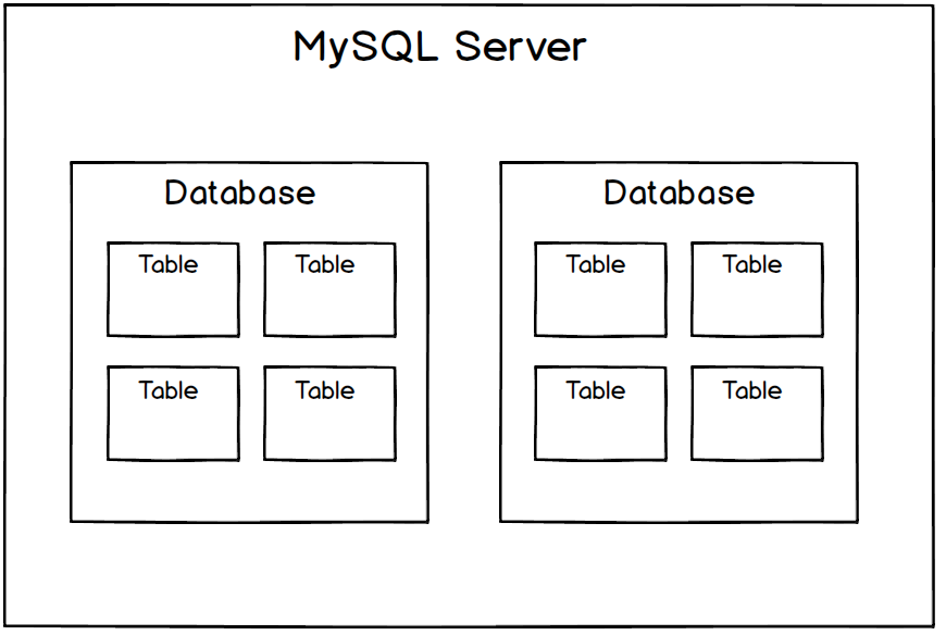
To query data from another database, you must prefix the database name. For example, if you are connected to the dvd database and want to query the baseball database, you must prefix table names with baseball.:
select * from baseball.batting;
To switch databases, run the use command:
use new_database;
Learn more
Someone dumped JSON into your database! {“uh”: “oh”, “anything”: “but json”}. What do you do?
Relational databases are beginning to support document types like JSON. It’s an easy, flexible data type to create but can be painful to query.
Here’s how to extract values from nested JSON in SQL 🔨:
Example
{"userId": "555", "transaction": {"id": "222", "sku": "ABC"}
Let’s select a column for each userId, id, and sku. The following queries return 555, 222, ABC.
Postgres
Use the ->> operator to extract a value as text, and the -> to extract a JSON object:
select
    my_json_field ->> 'userId',
    my_json_field -> 'transaction' ->> 'id',
    my_json_field -> 'transaction' ->> 'sku'
from my_table;
Redshift
Use the json_extract_path_text function:
select
    json_extract_path_text(my_json_field, 'userId'),
    json_extract_path_text(my_json_field, 'transaction', 'id'),
    json_extract_path_text(my_json_field, 'transaction', 'sku')
from my_table;
MySQL
MySQL 5.7 includes JSON support. Hurray! Use the json_extract function:
select
    json_extract(my_json_field, '$.userId'),
    json_extract(my_json_field, '$.transaction.id'),
    json_extract(my_json_field, '$.transaction.sku')
from my_table;
Learn more
- Querying JSON in Postgres
- JSON Docs: Postgres, Redshift, MySQL
What’s the easiest way to match case insensitive text anywhere in a string?
For example, let’s say you’re a fruit company marketing executive and you want all records matching “orange”, including “navel oranges”, “Syracuse Orange,” “Orange is the New Black”, “The Real Housewives of Orange County”, “orange you glad I didn’t say banana”, “🍊” and so on.
Here’s a quick way to match case insensitive text.
Postgres & Redshift
Use ~*:
select *
from my_table
where item ~* 'orange';
The ~* operator searches for ‘orange’ anywhere in the string, thanks to the power of regular expressions.
MySQL
Use like:
select *
from my_table
where item like '%orange%';
In MySQL, like is case insensitive and much faster than regexp (the MySQL equivalent of ~* in Postgres and Redshift). Add the % wildcard to both sides of ‘orange’ for a substring match.